Get Started • abslife

library(abslife)
#> Welcome to the abslife package!
#> WARNING: Under construction.
library(ggplot2) ## optional

This package is currently under construction!

This vignette demonstrates the core functionalities of the abslife package. abslife provides tools for estimation of the hazard rate, denoted \(\lambda\), for discrete time-to-event data subject to left-truncation (Lautier et al. 2023a). The package is designed so it can additionally handle the following common observational data challenges:

+ Right-censoring (Lautier et al. 2023b)
+ Competing risks (Lautier et al. 2024)

In all cases, asymptotic confidence intervals for the estimated hazard rates are readily available. The main function of the package is the estimate_hazard() function, which adapts to these scenarios based on the arguments provided.

Now, we provide specific examples with datasets shipped with the package.

Left-truncation

We begin by analyzing the aart dataset. This dataset represents a scenario involving only left-truncation. It contains two columns: Xi (time-to-event) and Yi (truncation time).

data(aart)
head(aart)
#>   Xi Yi credit.score interest.rate    pti veh.value co.sign new.used
#> 1 39 33          789        0.0290 0.1138  11.09935       0        1
#> 2 39 33          486        0.0499 0.0000  11.03240       0        1
#> 3 40 34          561        0.0250 0.0000  10.37246       0        1
#> 4 39 33          688        0.0259 0.0555  10.69326       0        1
#> 5 34 33          477        0.0490 0.0000  10.59031       0        1
#> 6 35 33          550        0.0239 0.0000  10.39776       0        1
#>   subvent.rate subvent.cash veh.pick.up veh.suv
#> 1            0            0           0       1
#> 2            0            1           1       0
#> 3            0            0           1       0
#> 4            0            1           1       0
#> 5            0            1           1       0
#> 6            0            0           1       0

We estimate the hazard rate using estimate_hazard().

aart_hazard <- estimate_hazard(lifetime = aart$Xi,
                               trunc_time = aart$Yi,
                               ci_level = 0.95,
                               carry_hazard = TRUE) ## need

Note that we set carry_hazard = TRUE. This argument ensures that if a hazard estimate is 0, it is replaced by the last non-zero estimate.

The function returns a data.frame containing the evaluation times, the hazard estimates, and the standard errors (on the log scale). It also includes the lower and upper bounds of the confidence interval corresponding to the ci_level argument (in this case, set to 0.95).

tail(aart_hazard)
#> Observed lifetime support: [36, 41] 
#> Total number of timepoints observed: 6

Summarizing and plotting

For a concise overview of the estimation, use the summary() method:

summary(aart_hazard)
#>    lifetime     hazard se_log_hazard    lower_ci   upper_ci
#> 1         5 0.01538462     0.7126096 0.003850968 0.05940167
#> 6        10 0.02183908     0.2319626 0.013972246 0.03398255
#> 11       15 0.02291826     0.1847030 0.016069256 0.03258974
#> 16       20 0.01963439     0.1875456 0.013677578 0.02811156
#> 21       25 0.02743902     0.1511595 0.020547920 0.03655493
#> 26       30 0.03096539     0.1422477 0.023609106 0.04051868
#> 31       35 0.04223676     0.1212668 0.033602069 0.05296869
#> 36       40 0.95017182     0.1905022 0.929214457 0.96515703

To visualize the hazard rate, you can use base R graphics via the plot() method:

plot(aart_hazard, ci_level = c(.5, .75, .85, .9, .95))

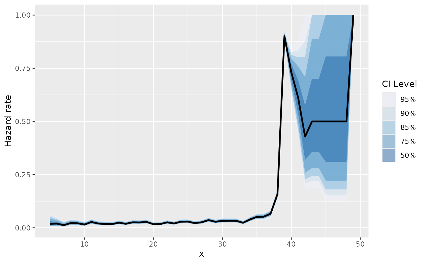
Alternatively, use ggauto() for a ggplot2-powered visualization. This function is particularly useful for visualizing multiple confidence levels simultaneously:

ggauto(aart_hazard, ci_level = c(.5, .75, .85, .9, .95))

Calculating the CDF

The package can also derive the Cumulative Distribution Function (CDF) directly from the hazard estimates using calc_cdf(). This appends a cdf column to the results.

aart_cdf <- calc_cdf(aart_hazard)
#> Warning in calc_cdf.alife(aart_hazard): Not reporting CDF (and density) values
#> for time points where the hazard rate equals 1.
summary(aart_cdf)
#>    lifetime        cdf    density
#> 1         5 0.01538462 0.01538462
#> 6        10 0.10437149 0.01999641
#> 11       15 0.20412422 0.01866792
#> 16       20 0.29434160 0.01413266
#> 21       25 0.37520875 0.01762734
#> 26       30 0.45948868 0.01727198
#> 31       35 0.55198866 0.01975702
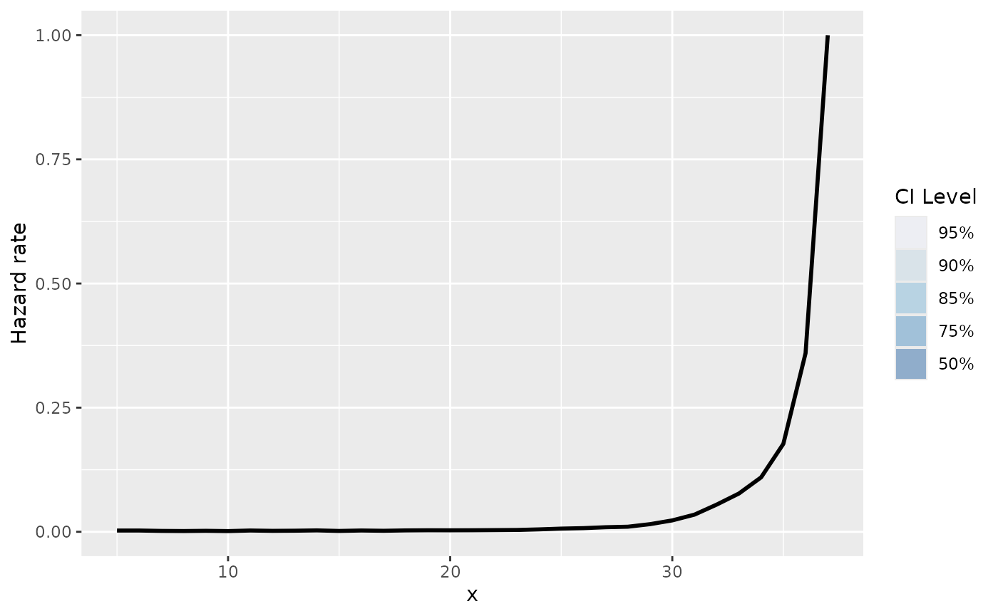
#> 36       40 0.99215705 0.14955687

We can also plot the CDF:

plot(aart_cdf)

Right-censoring

The workflow for right-censored data is nearly identical. We will demonstrate this using the mbalt dataset, which includes a third column, Di, serving as the right-censoring indicator.

data(mbalt)
head(mbalt)
#>   Zi Yi Di base.resid contract.resid co.lessee credit.score location lease.term
#> 1 37 29  1      24708       30139.20     FALSE          848       NJ         36
#> 2 30 29  1      18701       23466.30     FALSE          739       CA         36
#> 3 37 30  1      35571       36383.20      TRUE          871       NY         36
#> 4 32 32  1      30056       32342.76      TRUE          721       OH         36
#> 5 37 32  1      31489       33854.70      TRUE          738       NJ         36
#> 6 36 33  1      29319       30509.46     FALSE          736       CA         36
#>          pti subvented   model year  manufacturer veh.value
#> 1 0.04355511      cash  C300W4 2015 Mercedes-Benz     47090
#> 2 0.06285600      rate CLA250C 2014 Mercedes-Benz     35555
#> 3 0.04434177      none ML350W4 2015 Mercedes-Benz     64120
#> 4 0.04603333      rate ML350W4 2014 Mercedes-Benz     58995
#> 5 0.00514451      rate ML350W4 2015 Mercedes-Benz     60655
#> 6 0.05854000      rate ML350W2 2014 Mercedes-Benz     55600

We call estimate_hazard() again, but this time we provide the censoring argument. This argument accepts a vector where 1 indicates a censored observation and 0 indicates an observed event.

mbalt_hazard <- estimate_hazard(lifetime = mbalt$Zi,
                                trunc_time = mbalt$Yi,
                                censoring = 1 - mbalt$Di,
                                ci_level = 0.95,
                                carry_hazard = FALSE) ## need

The output structure remains consistent with the previous example.

summary(mbalt_hazard)
#>    lifetime      hazard se_log_hazard     lower_ci    upper_ci
#> 1         5 0.002508511    0.26759709 0.0014862156 0.004231014
#> 6        10 0.001434226    0.20014358 0.0009692981 0.002121686
#> 11       15 0.001737202    0.14599186 0.0013054782 0.002311367
#> 16       20 0.002970186    0.09727315 0.0024558880 0.003591798
#> 21       25 0.006408331    0.06270123 0.0056714682 0.007240233
#> 26       30 0.022951745    0.03238300 0.0215707217 0.024418979
#> 31       35 0.177075260    0.01673112 0.1723472557 0.181904461

The plotting functions also work out of the box:

plot(mbalt_hazard)

and, for ggplot2:

ggauto(mbalt_hazard, ci_level = c(.5, .75, .85, .9, .95))

Competing risks

Finally, abslife can estimate hazards in the presence of competing risks. We use the aloans dataset, which contains data on consumer automobile loans (Lautier et al. 2024).

data(aloans)
head(aloans)
#>     risk.cat  Z  Y C D R bond orig.apr orig.term orig.loan.amt cur.age
#> 1      prime 36 18 0 0 1 aart   0.0704        72      13649.18      17
#> 2 near_prime 60 17 1 0 0 aart   0.1025        72      19999.10      16
#> 3      prime 28 17 0 0 1 aart   0.0694        72       9098.58      16
#> 4 near_prime 33 17 0 0 1 aart   0.1080        72      11723.36      16
#> 5      prime 60 17 1 0 0 aart   0.0869        72       8753.48      16
#> 6      prime 46 17 0 0 1 aart   0.0560        72      22206.59      16
#>   cur.balance calc.pmt
#> 1    11448.24 231.5438
#> 2    16143.29 368.4643
#> 3     7600.87 153.9386
#> 4     9665.35 218.9605
#> 5     7515.89 155.0285
#> 6    18458.99 362.4058

The relevant columns of the dataset for this example are the following:

Z: time to event
Y: left-truncation
C: right censoring indicator
D: Default indicator (1 represents default, and 0 represents pre-payment)

The two competing risks in this case are default and pre-payment. To make the results more interpretable, we create a descriptive event_type column.

aloans <- transform(aloans, event_type = ifelse(D == 1, "Defaut", "Pre-payment"))

The package is designed so the workflow is identical as the previous two examples. The only change here is passing the column discriminating the event types to the event_type argument in estimate_hazard().

aloans_hazard <- estimate_hazard(lifetime = aloans$Z,
                                 trunc_time = aloans$Y,
                                 censoring = aloans$C,
                                 event_type = aloans$event_type,
                                 ci_level = 0.95,
                                 carry_hazard = FALSE) ## need 
#> Warning in check_censored(lifetime, censoring_indicator, support_lifetime_rv):
#> Warning: Detected censored observations at the maximum limit of the support
#> (lifetime == max(support_lifetime_rv)). This may lead to identifiability issues
#> or unstable hazard estimates at the tail.

The output now includes a column specifying the event type for each hazard estimate.

summary(aloans_hazard)
#>     event_type lifetime      hazard se_log_hazard    lower_ci    upper_ci
#> 1       Defaut        3 0.011520293    0.06506047 0.010155080 0.013066617
#> 2       Defaut        8 0.012729470    0.03876609 0.011809112 0.013720562
#> 3       Defaut       13 0.010477761    0.04486786 0.009604176 0.011429888
#> 4       Defaut       18 0.013350256    0.04224199 0.012302520 0.014485913
#> 5       Defaut       23 0.012722853    0.04637351 0.011630319 0.013916572
#> 6       Defaut       28 0.013859145    0.04731310 0.012647271 0.015185355
#> 7       Defaut       33 0.013032176    0.05225905 0.011778374 0.014417499
#> 8       Defaut       38 0.018664205    0.04681281 0.017055857 0.020421067
#> 9       Defaut       43 0.011084154    0.06587830 0.009754619 0.012592597
#> 10      Defaut       48 0.007673623    0.08514621 0.006501842 0.009054661
#> 11      Defaut       53 0.006133755    0.10401466 0.005008188 0.007510380
#> 12      Defaut       58 0.006600660    0.50165838 0.002479550 0.017451386
#> 13      Defaut       63 0.000000000    0.00000000 0.000000000 0.000000000
#> 14      Defaut       68 0.000000000    0.00000000 0.000000000 0.000000000
#> 15 Pre-payment        3 0.000000000    0.00000000 0.000000000 0.000000000
#> 16 Pre-payment        8 0.007686787    0.04975978 0.006977496 0.008467566
#> 17 Pre-payment       13 0.011646595    0.04258207 0.010724035 0.012647505
#> 18 Pre-payment       18 0.015630141    0.03908499 0.014494211 0.016853574
#> 19 Pre-payment       23 0.011372231    0.04901653 0.010341306 0.012504631
#> 20 Pre-payment       28 0.015052316    0.04542667 0.013787747 0.016430935
#> 21 Pre-payment       33 0.015385696    0.04815372 0.014019446 0.016882814
#> 22 Pre-payment       38 0.013687084    0.05452748 0.012316859 0.015207396
#> 23 Pre-payment       43 0.018648019    0.05098525 0.016904597 0.020567482
#> 24 Pre-payment       48 0.017776306    0.05622984 0.015950891 0.019806416
#> 25 Pre-payment       53 0.032053819    0.04610587 0.029365598 0.034979259
#> 26 Pre-payment       58 0.037953795    0.21258769 0.025348580 0.056464133
#> 27 Pre-payment       63 0.020408163    1.01036297 0.002867406 0.131138926
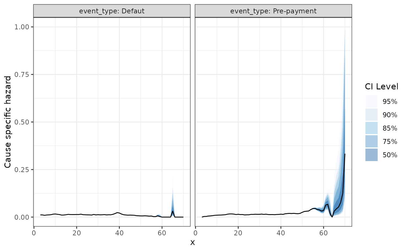
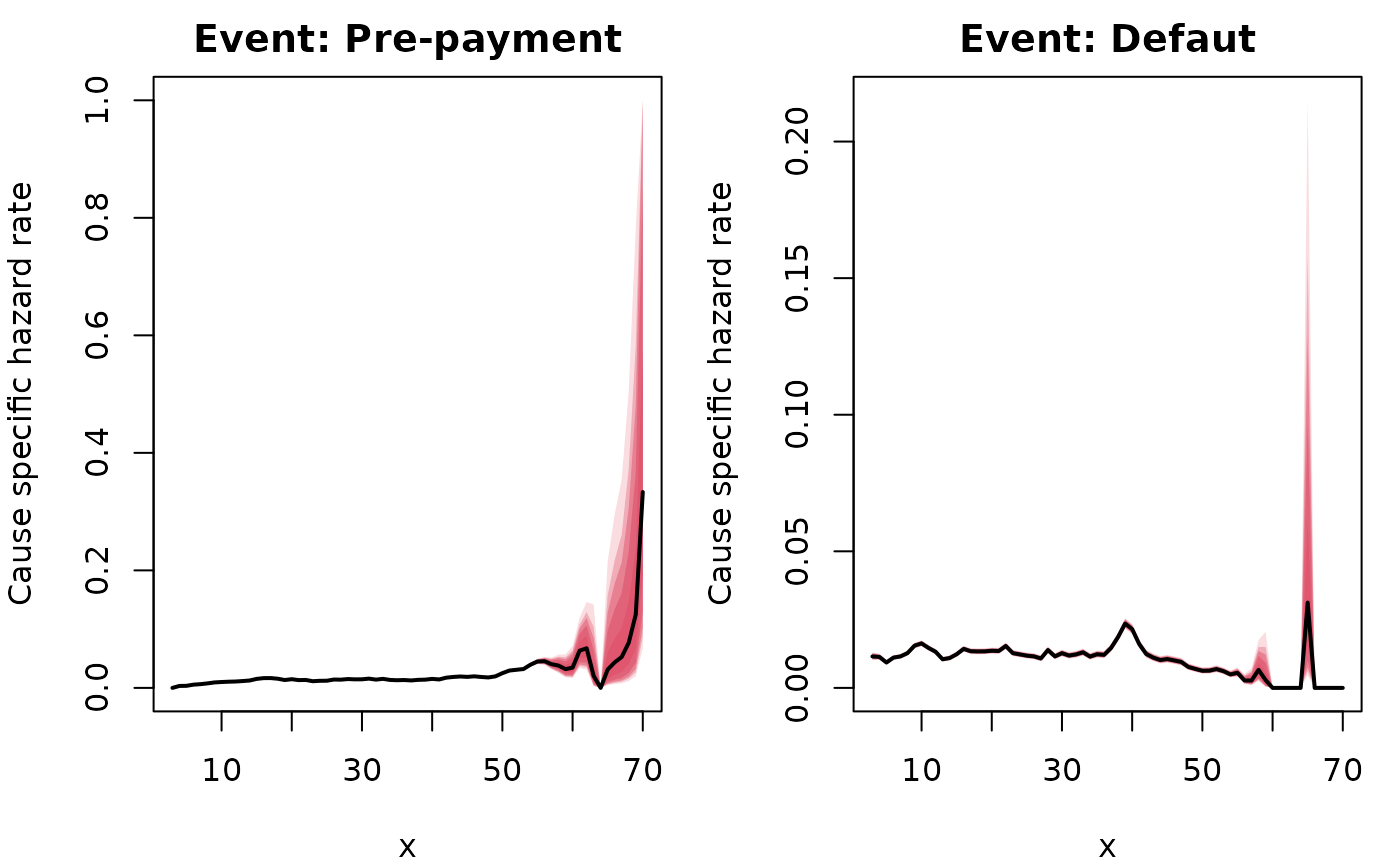
#> 28 Pre-payment       68 0.076923077    1.04083300 0.010719623 0.390571292

The plotting functions work as in the previous examples, handling the stratification by event type automatically:

plot(aloans_hazard, ci_level = c(.5, .75, .85, .9, .95))

The same holds for the ggplot2 powered plots:

ggauto(aloans_hazard, ci_level = c(.5, .75, .85, .9, .95)) +
  theme_bw()

References

Lautier, Jackson P., Vladimir Pozdnyakov, and Jun Yan. 2023a. “Estimating a Discrete Distribution Subject to Random Left-Truncation with an Application to Structured Finance.” Econometrics and Statistics, ahead of print. https://doi.org/10.1016/j.ecosta.2023.05.005.

Lautier, Jackson P., Vladimir Pozdnyakov, and Jun Yan. 2023b. “Pricing Time-to-Event Contingent Cash Flows: A Discrete-Time Survival Analysis Approach.” Insurance: Mathematics and Economics 110: 53–71. https://doi.org/10.1016/j.insmatheco.2023.02.003.

Lautier, Jackson P, Vladimir Pozdnyakov, and Jun Yan. 2024. “On the Convergence of Credit Risk in Current Consumer Automobile Loans.” Journal of the Royal Statistical Society Series A: Statistics in Society, December, qnae137. https://doi.org/10.1093/jrsssa/qnae137.