3. Areal Interpolation

In applied settings, estimating socioeconomic and demographic variables for different administrative regions within a city is often of interest. While areal interpolation (AI, Goodchild and Lam 1980) easily computes such estimates, it lacks measures of uncertainty (Bradley, Wikle, and Holan 2016). Our package addresses this by providing both areal interpolation and methods to approximate the variance of estimates when the observed data’s variance is known, as is common with survey data.

This demonstration will utilize 2010 Brazilian Census data from Nova Lima. The objective is to estimate some variables in a separate map of the same municipality. The census map with the original data will be referred to as the “source” map, while the map where the data will be estimated will be referred to as the “target” map. In this example, the target map is artificially generated. To initiate the process, the data and necessary packages can be loaded using the code below. We recommend using a planar Coordinate Reference System (CRS) when using this method.

library(sf)
#> Linking to GEOS 3.10.2, GDAL 3.4.1, PROJ 8.2.1; sf_use_s2() is TRUE
library(smile)
library(ggplot2)

data(nl_ct)
nl_ct <- st_transform(nl_ct, 20823)

The code chunk below creates the synthetic target map.

set.seed(2024)

## outer polygon
nl_outer <- nl_ct |>
  st_geometry() |>
  st_union() |>
  smile:::st_remove_holes()

## creating `target` data
points_nl <- st_sample(x = nl_outer,
                       size = 40)

nl_vor <- do.call(c, points_nl) |>
  ## voronoi tesselation
  st_voronoi(envelope = nl_outer) |> 
  st_collection_extract(type = "POLYGON") |>
  st_set_crs(st_crs(nl_ct)) |>
  st_intersection(nl_outer) |>
  st_as_sf()

## creating id variable
nl_vor <- transform(nl_vor, id = seq_len(NROW(nl_vor)))

Now, to estimate one (or several) variable observed at the nl_ct dataset into the nl_vor data we can run the following command:

nl_ests <-
    ai(source = nl_ct,
       target = nl_vor,
       vars = c("hh_density",
                "avg_income",
                "avg_age"))

## displaying the result
nl_ests |>
  st_drop_geometry() |>
  head()
#>   id hh_density avg_income  avg_age
#> 1  1   2.695228   1730.009 24.02146
#> 2  2   2.477646   2078.178 25.59811
#> 3  3   3.154861   1729.689 30.22053
#> 4  4   2.920528   2253.925 30.70541
#> 5  5   3.300867   7904.903 34.49821
#> 6  6   3.390798   5468.113 34.89071

In the function above, source is the map/dataset where the variables to be estimated are observed, while target is the map/dataset where the estimation is desired. The vars argument is a character scalar (or vector) specifying the variable(s) in source to be estimated in target. However, this function does not quantify uncertainty in the estimates.

If the variance of the variable we wish to estimate in the target map is available in the source map, we can use the ai_var function to quantify the uncertainty around our point estimates. The function is similar to ai, but with a few differences:

1. vars must be a single variable name.

2. my_var is a character indicating the variable in source containing the observed variable’s variance.

3. var_method specifies the method for approximating variance: Moran’s I (“MI”) for autocorrelation-based approximation, or Cauchy-Schwarz (“CS”) for an upper bound.

4. The current version only supports one variable at a time.

The ai_var function outputs the target dataset with two additional columns: est (estimated variable) and se_est (approximate standard error).

nl_est <-
    ai_var(source = nl_ct,
           target = nl_vor,
           vars = "hh_density",
           vars_var = "var_hhd",
           var_method = "MI")

## renaming geometry
st_geometry(nl_est) <- "geometry"

Below we use ggplot2 to plot the observed and estimated “household density” in the source and target maps, respectively.

viz_dt <-
    rbind(
        transform(nl_ct, source = "Observed",
                  est = hh_density)[c("source", "est")],
        transform(nl_est, source = "Estimated")[c("source", "est")]
    )

ggplot(data = viz_dt,
       aes(fill = est)) +
    geom_sf(color = 1, lwd = .1) +
    scale_fill_viridis_c(option = "H",
                         name = "Household \n density") +
    theme_bw() +
    facet_wrap( ~ source) +
    theme(axis.text = element_blank(),
          axis.ticks = element_blank())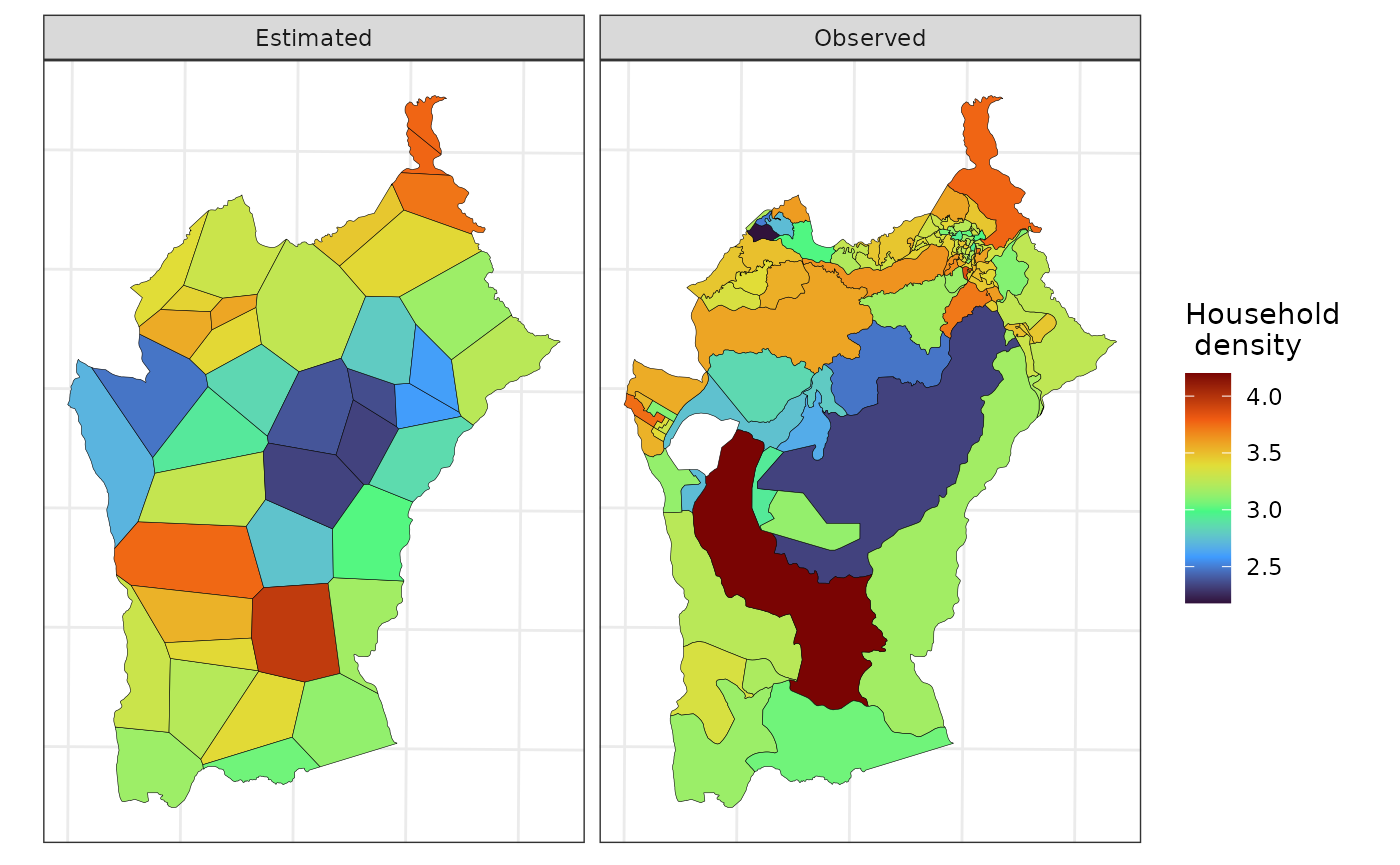

Finally, the next map displays the uncertainty about the estimated household density.

Reference

Bradley, Jonathan R., Christopher K. Wikle, and Scott H. Holan. 2016. “Bayesian Spatial Change of Support for Count-Valued Survey Data with Application to the American Community Survey.” Journal of the American Statistical Association 111 (514): 472–87. https://doi.org/10.1080/01621459.2015.1117471.

Goodchild, Michael F, and Nina Siu-Ngan Lam. 1980. “Areal Interpolation: A Variant of the Traditional Spatial Problem.” Geo-Processing 1: 279–312.