library(smile)
library(ggplot2)
library(sf)
#> Linking to GEOS 3.12.1, GDAL 3.8.4, PROJ 9.4.0; sf_use_s2() is TRUE
Spatial data often needs to be analyzed at different scales or resolutions. This package helps you align disparate spatial data using two approaches:
Model-based: This approach is based on the assumption that areal data (e.g., variables measured at census tracts) are composed by averages of a continuous underlying process (Gelfand, Zhu, and Carlin 2001). In particular, we assume this underlying process to be a Gaussian Process Johnson, Diggle, and Giorgi (2020).
Non-parametric spatial interpolation: This simpler method estimates values at a new spatial support based on the area of intersection between areal units. If you are interested in the non-parametric approach, visit our vignette on the topic.
This vignette focuses on the model-based approach for areal data
(like, for instance, census tract data). This method involves converting
sf(Pebesma 2018) objects (a
common format for spatial data in R) to the spm format used by this
package. We’ll use the ggplot2(Wickham 2011) package for visualization.
To demonstrate this conversion, we’ll use life expectancy at birth (LEB) and the index of multiple deprivation (IMD) data for Liverpool from Johnson, Diggle, and Giorgi (2020). This data is available at different spatial resolutions (MSOA and LSOA). See Figure for a visualization of life expectancy at the MSOA level.
data(liv_lsoa) # loading the LSOA data
data(liv_msoa) # loading the MSOA data

## workaround for compatibility with different PROJ versions
st_crs(liv_msoa) <-
    st_crs(liv_msoa)$input
st_crs(liv_lsoa) <-
    st_crs(liv_lsoa)$input
ggplot(data = liv_msoa,
       aes(fill = leb_est)) +
    geom_sf(color = "black",
            lwd   = .1) +
    scale_fill_viridis_b(option = "H") +
    theme_minimal()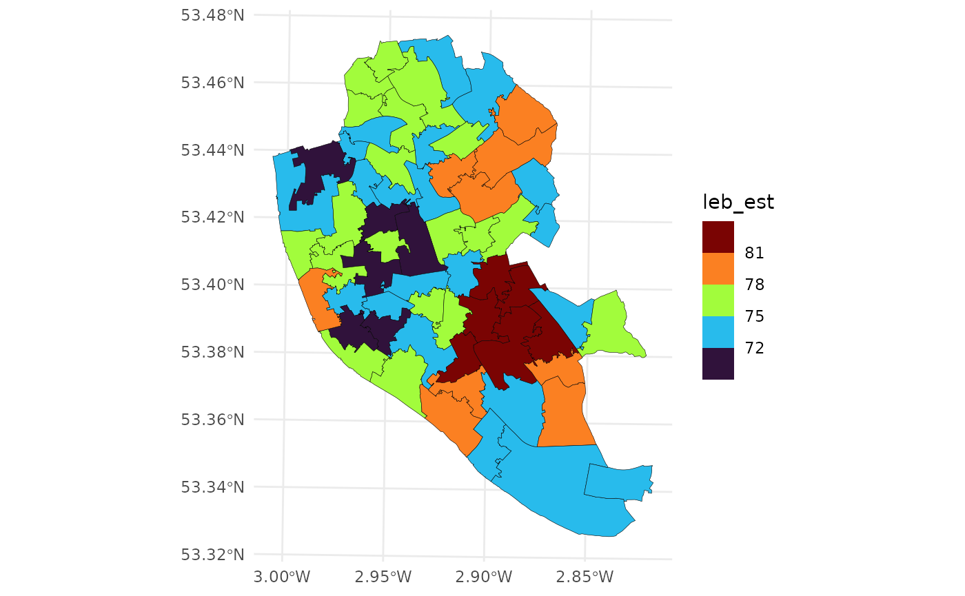
LEB in Liverpool at the MSOA.
To analyze the relationship between life expectancy (LEB) and deprivation at the LSOA level, we need to estimate LEB at this higher resolution. We assume LEB follows a continuous spatial pattern represented by a Gaussian process.
Mathematically, the observed LEB in an areal resolution (e.g., an MSOA) as averages of a continuous underlying process across that area. If we knew the exact parameters of this process, we could calculate the LEB for any location. However, these calculations involve complex integrals that are difficult to solve analytically. For more details on the theory behind this, see this vignette.
The sf_to_spm function controls how the model-based
approach will approximate these integrals. It supports either numerical
or Monte Carlo integration. Here’s how different parameters of this
function change the integration method:
type: Controls the grid used for approximating the integrals. Options include “regular”, “hexagonal” (both for numerical integration), and “random” (for Monte Carlo integration).npts: Specifies the number of grid points used to approximate the integral. This can be a single value or a vector with different values for each area. More points generally improve accuracy but increase computation time.-
by_polygon: Determines if the precision of the approximation should vary by polygon size.-
TRUE: All integrals are estimated with the same precision. -
FALSE: A grid of points is generated over the entire region, and points are assigned to the areas they fall within. This results in more points and higher accuracy for larger polygons.
-
This approach allows us to estimate LEB at the LSOA level while accounting for the underlying spatial structure of the data.
The code below converts the liv_msoa object (in
sf format) to an spm object. We generate a
grid of 1000 points across Liverpool and assign each point to its
corresponding area.
msoa_spm <-
    sf_to_spm(sf_obj = liv_msoa, n_pts = 1000,
              type = "regular", by_polygon = FALSE,
              poly_ids = "msoa11cd", var_ids = "leb_est")
Here’s what the additional arguments of the sf_to_spm
function do:
poly_ids: Specifies the column in liv_msoa that contains the unique identifier for each area (e.g., an area ID).var_ids: Indicates the column containing the “response variable” – the variable we want to model (e.g., life expectancy).
This conversion prepares the data for spatial analysis using the
smile package.
type and by_polygon when calling the
sf_to_spm function.
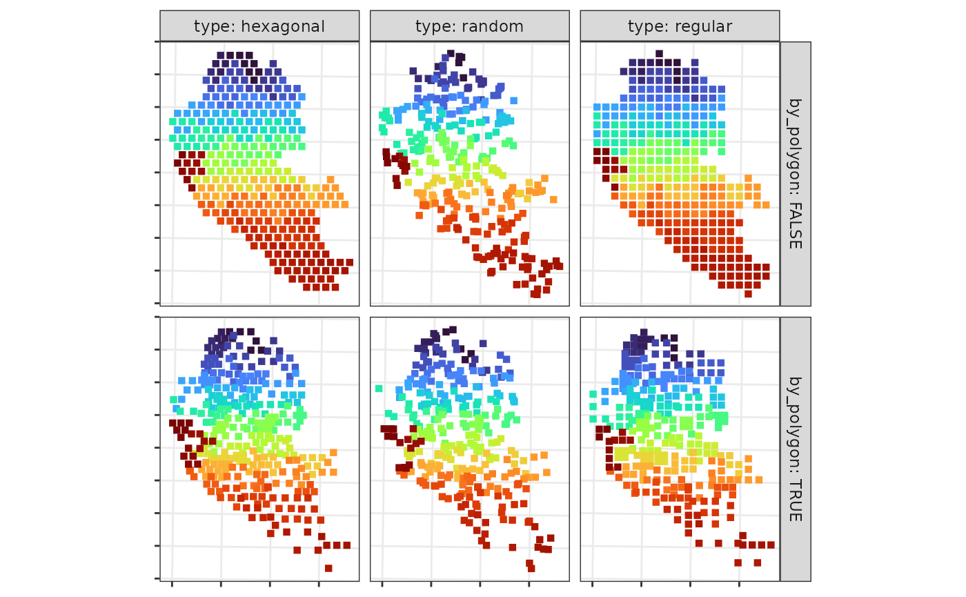
Panel illustrating the grids generated for different approaches to approximate numerical integrals in the model-based approach.
For details on fitting models and making predictions, see this vignette.